Astrophysical calibration using two exceptional black hole mergers
The LIGO, Virgo and KAGRA (LVK) Collaboration has detected more than 300 gravitational-wave signals from coalescing black holes and neutron stars. Each signal encodes information about its source and the extreme physics that governs these collisions. Extracting this information requires the gravitational-wave observatories to detect the gravitational-wave emission precisely (hearing the signals clearly, in a sense), and account for any uncertainties in their measurements. The LVK Collaboration reports two new loud gravitational-wave signals, GW240925 and GW250207, with which we are able to perform the first informative tests of astrophysical calibration.
It was a surprisingly good kind of bad timing: we observed two loud gravitational-wave signals (see Figure 1) at times when the LIGO Hanford detector was, metaphorically, out of tune – meaning we do not precisely know how to interpret its data. But thanks to the loudness of the signals, we are able to analyse them and tune LIGO Hanford by directly measuring the state of the detector at the same time. This is particularly important in the case of GW250207, for which the detector uncertainty is largely unknown and changing with time.
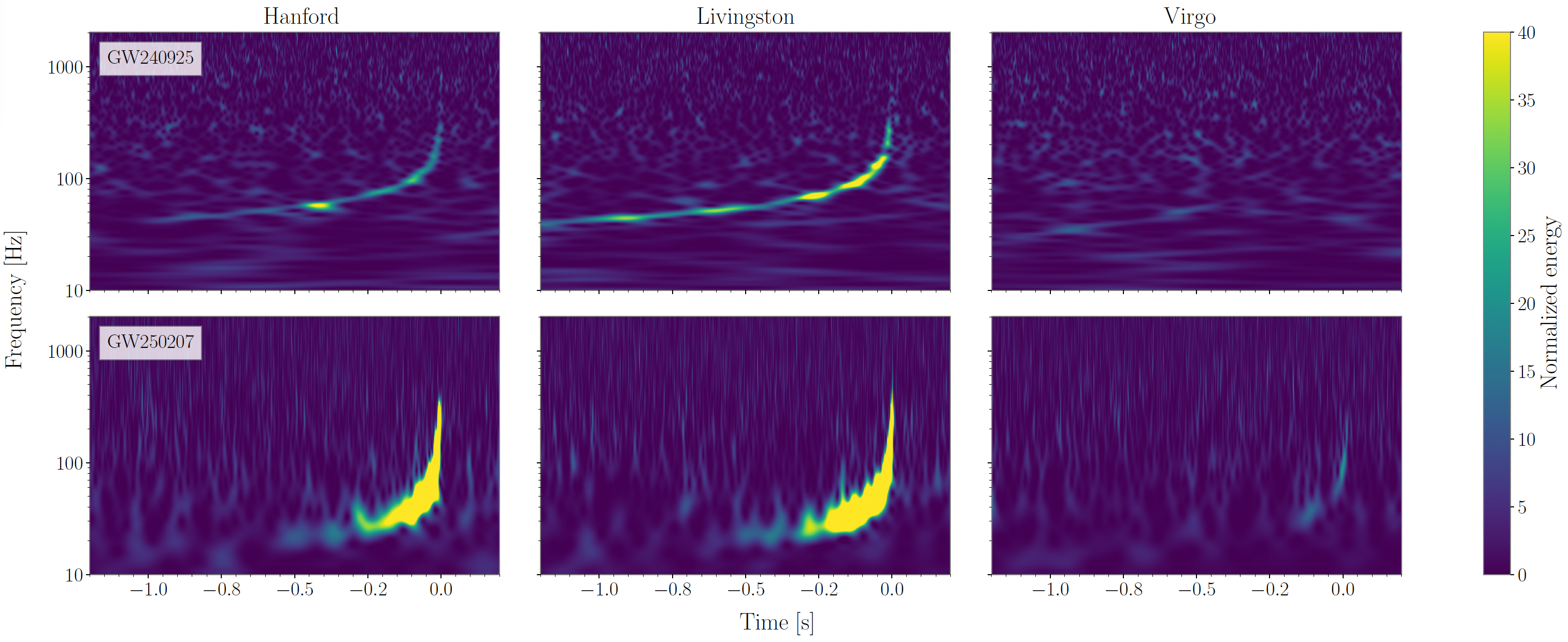
Figure 1: The gravitational-wave events GW240924 (top row) and GW250207 (bottom row) as observed by the LIGO Hanford (left column), LIGO Livingston (middle column), and Virgo (right column) observatories. The plots, called spectrograms, show the power spectrum (energy at different frequencies) as a function of time. The signals can be seen as the increase in energy over time (in seconds) and at specific frequencies (in hertz), represented by green and yellow bands. Their shape follows the characteristic chirp pattern produced by gravitational-wave signals. The thickness and brightness of GW250207 shows just how loud it was!
Astrophysical calibration
Gravitational waves stretch and squeeze spacetime as they pass by. The LVK detectors measure this by sending laser light down two perpendicular arms and looking for tiny differences in the light’s travel time – evidence that the arm lengths have changed. The typical gravitational-wave will change the arm length by around 10-19 m, that’s much smaller than the width of a proton! In order to stay sensitive to such small changes, we carefully regulate the detectors in real time, using feedback control loops. Now, not only do we need to convert from the light travel time to a signal, we have to account for how the control loops changed the light travel time as well. This is done through a careful calibration procedure that models how the detector changes as the waves move through (yes, including the control loops!). Generally, we cannot create a perfect model and have to correct our measurements by calculating the mismatch between our model and the true model. We can do this by looking at the errors and uncertainties in our calculations. We quantify the mismatch using auxiliary lasers and sensors and our detailed knowledge of the instrument. But what happens when that extra information is not available, and a proper calibration cannot be performed?
If the calibration is inaccurate, the source information we infer may be biased, which can lead us to draw the wrong conclusions about the physics involved. Fortunately, if a gravitational-wave signal is loud enough, it can be disentangled from the calibration error. If we assume Einstein’s theory of general relativity predicts what the signal should look like correctly, we can mitigate potential biases in the results. This is called astrophysical calibration. For both the GW240925 and GW250207 detections, we can employ our usual methods to estimate the calibration errors for the LIGO Livingston and Virgo detectors, but not for the LIGO Hanford detector. Thankfully, both signals are sufficiently loud to perform the very first informative tests of astrophysical calibration! The probable shapes of the calibration errors we find are shown in Figure 2. A summary of both events is given in Table 1.
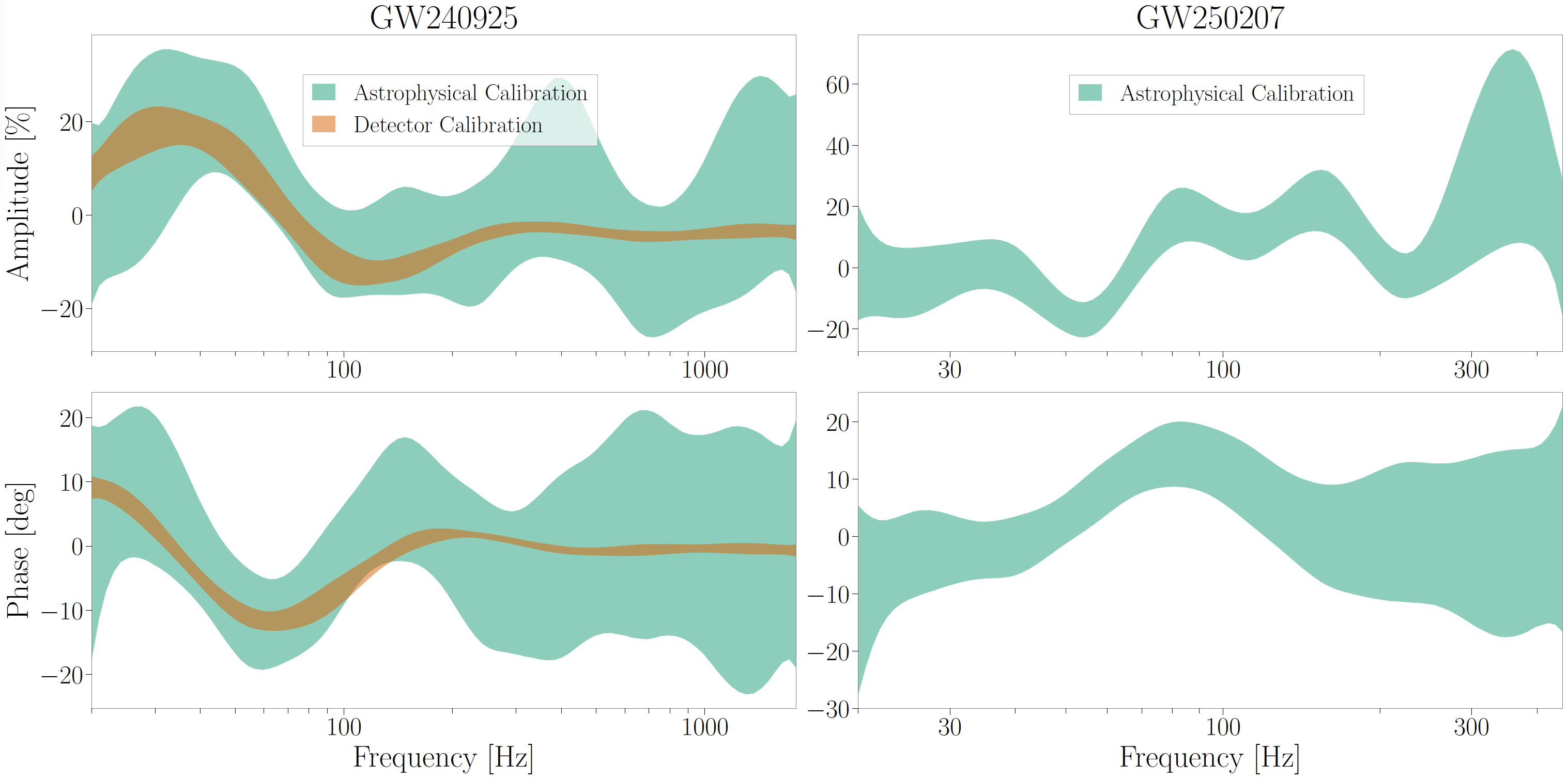
Figure 2: The probable shape of the inferred Hanford calibration error in terms of its amplitude and phase as a function of frequency. The larger the shaded region for a certain frequency, the larger our uncertainty as to what exactly the calibration error is there. The plots for GW240925 on the left show in green the results from the astrophysical calibration on the initial data, and in orange the quantified error using extra information measured in the detector (referred to as the ‘Detector Calibration’). We can see that the green-shaded region encapsulates the orange, which means we are successfully inferring the shape of the calibration error! On the right, we have the GW250207 results with only the green-shaded region as there was no extra detector information to cross-check these results with.
| GW240925 | GW250207 |
| A technical issue in the Hanford detector created a temporary miscalibration of the live data, which was quantified and fixed at a later stage, allowing correctly calibrated data to be produced offline. This means we can perform astrophysical calibration on the initial data, and compare analysis results between this and the final correctly-calibrated data. | During this signal, LIGO Hanford had just been turned on and was in an unsettled state. Several auxiliary sensors were not collecting data, making it impossible to calculate the calibration error. This is the second loudest event we’ve ever observed, and it provides a unique window into some exciting physics. Accessing this information is only possible thanks to astrophysical calibration measurements of the calibration error. |
Table 1: Brief summary of the observational context for GW240925 and GW250207.
Why is astrophysical calibration important?
With accurate gravitational-wave data we can estimate the properties (or parameters) of the black holes that generated the gravitational-wave signal, properties such as the masses of the black holes, whether they are spinning or not, and where in the sky they are located (sky localization). We find that GW240925 was generated by black holes of 9 and 7 times the mass of the Sun at a distance of ~350 megaparsecs from the Earth, and GW250207 by two black holes of 35 and 30 times the mass of the Sun at a distance of ~200 megaparsecs from the Earth; neither event provides much evidence that the black holes were rapidly spinning. Without properly accounting for calibration uncertainties, these estimates could be biased towards a value that is not true, so we require accurate calibration uncertainties to ensure that we can trust the data.
We can also use the gravitational-wave data and the estimated source parameters to perform exciting analyses such as testing general relativity and determining the Hubble constant. General relativity is Einstein’s theory of gravity; testing it in extreme situations, such as during the merger of two black holes, means we can see whether there are any discrepancies between what the theory predicts and what we observe. While we have yet to find a discrepancy between general relativity and observations, it is not a complete theory and understanding where observations differ from its predictions may enable us to come up with a new, more complete, theory. While calibration errors cannot mimic gravitational-wave signals, they could mimic deviations from general relativity. So our confidence in a possible discrepancy between general relativity and our observations could be undermined by calibration errors, meaning we cannot trust our interpretation of the data! In cases such as GW250207, where typical methods of calibration were unavailable, we can use astrophysical calibration instead, so that we can still trust the data. When using astrophysically-calibrated data, no discrepancy between Einstein’s theory and the observations was detected for this event.
Using astrophysical calibration, so that we can trust the data from the LIGO Hanford detector, also means that we can narrow down the area we believe the gravitational-waves originated from. This sky localization works in a similar way to triangulation, where the more detectors involved in a detection, the more we can narrow down the area of likely origin for the signal. In Figure 3, the possible area significantly shifts and shrinks when correctly-calibrated LIGO Hanford data is used.
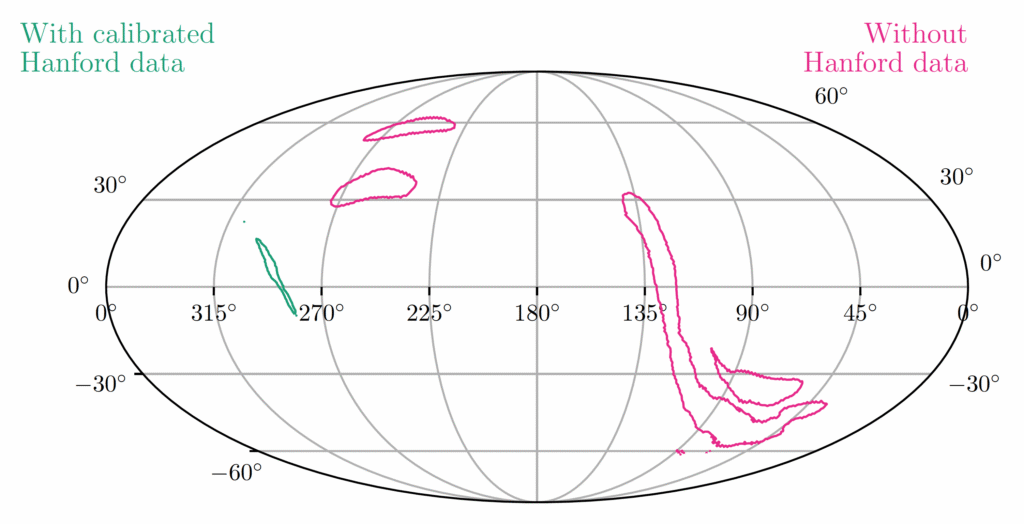
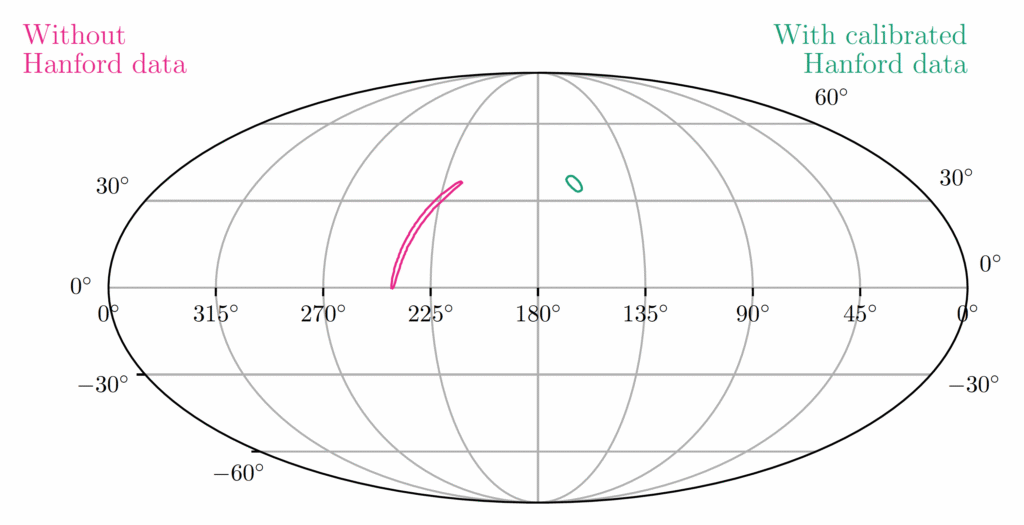
Figure 3: Sky localisation of GW240925 (left) and GW250207 (right). The pink areas are obtained using data from the LIGO Livingston and Virgo detectors. Using the astrophysically-calibrated LIGO Hanford data, the possible source location shifts and shrinks to the green area.
Sky localization is a key ingredient in the measurement of the Hubble constant, a value that can tell us the rate of expansion of the Universe. To determine the Hubble constant, we need to measure cosmic distances. The two main methods to do this are measuring the brightness of standard candles such as supernovae, and measuring fluctuations in the cosmic microwave background radiation that is left over from the big bang. However, these methods do not agree on the value of the constant, leading to the Hubble tension. Using gravitational-waves to measure the Hubble constant may help resolve this tension. Due to its position in the sky and loudness, GW250207 is thought to be one of the best binary black hole signals to measure the Hubble constant but it is unable to resolve the tension alone as many more such dark sirens would be required to produce an accurate measurement of the Hubble constant. Analysis of all dark sirens detected during the first part of the fourth observing run is covered in this previous science summary.
GW240925 and GW250207 have allowed us to perform the first informative tests of astrophysical calibration, a new possible calibration method for loud signals that could help us trust our data even when the gravitational-wave detectors are in an unsettled state, allowing us to apply it to enhance our ability to measure source properties, test Einstein’s theory of gravity and determine the rate of expansion of the Universe using gravitational waves!
Find out more
- Visit our websites:
- Read the full scientific article: https://doi.org/10.1103/gzrj-mwv3 or on arxiv: https://arxiv.org/abs/2605.11703
- Gravitational-Wave Open Science Centre data release:
- Data for GW240925:https://doi.org/10.7935/d2tg-qv58
- Data for GW250207:https://doi.org/10.7935/k8et-b503
- Zenodo data release: https://doi.org/10.5281/zenodo.18600070
Back to the overview of science summaries.