The third observing run (O3) of the Advanced LIGO and Advanced Virgo detectors ended in March 2020. During O3 several tens of Gravitational Waves (GWs) have been confirmed, originating from the compact binary coalescence (CBC) of Black Holes and/or Neutron Stars. However, CBCs are only one type of GW sources among a wider range of possibilities. Here we focus on a type of GW transients that have particularly short time duration (less than 1 second): we also call these “short bursts”. Potential examples of short burst sources (besides binary black hole mergers) include core-collapse supernovae, cosmic string cusps, or pulsar glitches — as well as the exciting possibility of totally new unpredicted sources.
Unmodeled Searches
Given the lack of precise models for most of these potential sources, it is important to process the data with algorithms capable of detecting almost any type of signal, as long as it is short: this is a so-called “unmodeled” short-duration transient search. Compared to the dedicated CBC search approach, where we search in the data for features corresponding to known waveform ‘templates’, an unmodeled search extracts excesses in the data which could be compatible with GWs satisfying minimal assumptions. However, the downside to this unmodeled approach is that these search algorithms are limited by the presence of noise artifacts (detector glitches – not to be confused with pulsar glitches) in the data, which can resemble a genuine GW signal. Thanks to the information from auxiliary channels, which monitor the external and internal state of the interferometers, a large fraction of these detector glitches can be identified and vetoed. This helps to improve the statistical significance of possible candidates.
Two search algorithms have been considered for this work: coherent Waveburst (cWB) extracts a list of GW signal candidates from the data, and BayesWave (BW) performs a follow-up analysis of the cWB candidates. The two algorithms have been tested on a set of ad-hoc simulated waveforms where a few different generic signal ‘shapes’ have been added to the data to determine how energetic a GW must be to be observable by our detectors.
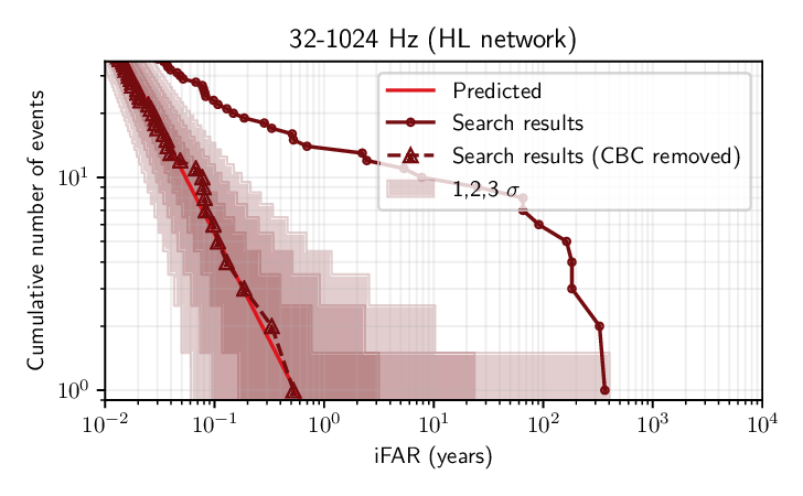
Figure 1 (figure 2 in the paper): Cumulative number of events (vertical axis) shown against the probability of being generated randomly by noise excesses (expressed as inverse false alarm rate in years, horizontal axis). Two sets of symbols connected with lines show the total number found by the search (circular points) and after having discarded all known CBC sources from the data (triangular points). The solid line represents the expected noise-only background and shaded regions indicate its statistical uncertainty.
Results
Figure 1 shows the list of candidates from the search, compared with the expected distribution in the case where they come from noise excesses. The predicted distribution is obtained with the widely used procedure of time-shifting detector data. No new GW candidates have been found, apart from some of the already detected CBC sources (the ones that imprint a short-duration signal in the data, corresponding to massive compact objects). While in the previous runs we characterized the sensitivity of similar searches by considering ad-hoc generic waveforms, in this work we additionally investigate how well the search is able to detect two specific possible astrophysical sources: core-collapse supernovae (CCSN) and isolated neutron stars (NS).
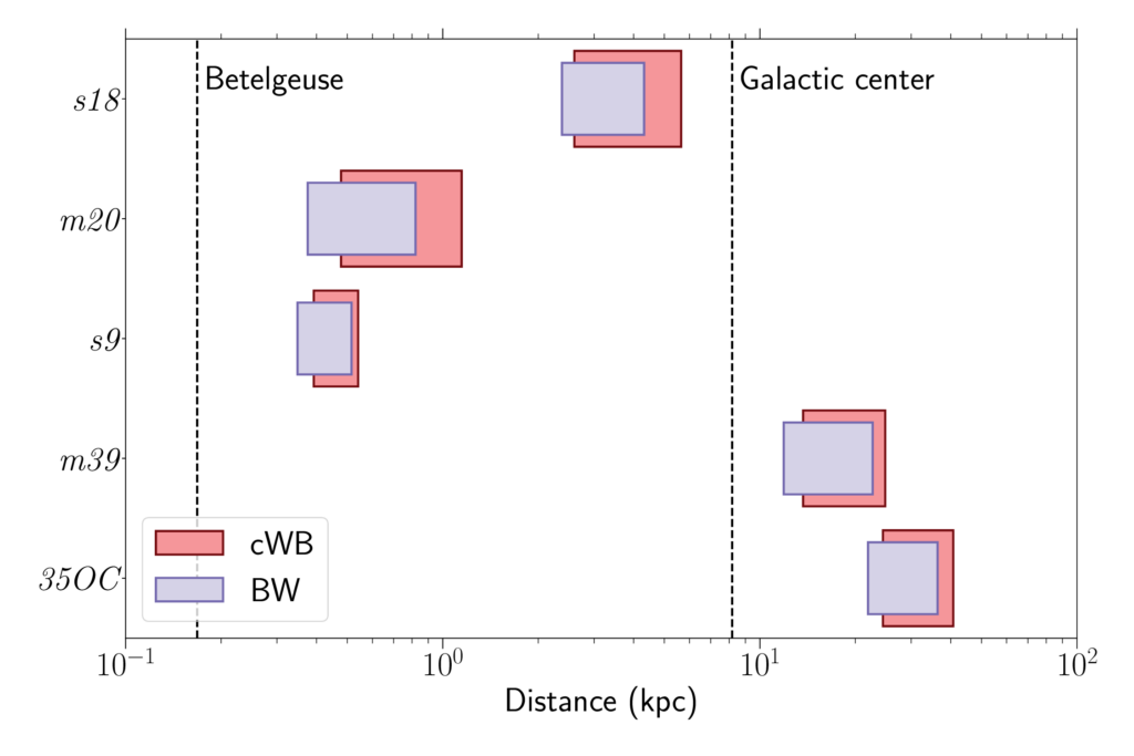
Figure 2 (figure 7 in the paper): Distances of a source from Earth at which our algorithms can detect different CCSN waveforms. The left edge of each box refers to the distance (in thousands of parsecs, denoted kpc) at which we detect 10% of the signals, while the right edge shows the distance corresponding to 50% efficiency. The vertical axis refers to different CCSN waveforms; see the paper for more details on the models considered. Different colors represent results from the two detection algorithms used.
Figure 2 shows the distance ranges from Earth within which our searches would detect a CCSN with an efficiency between 10 and 50%, depending on different GW emission models. We also want to know how large a pulsar glitch would need to be, in order to be detected in our data. Figure 3 shows the size of pulsar glitch that could be detected with an efficiency of 50%, assuming various emission models described by different equations of state and considering as a reference the distance and spin of the Vela pulsar.
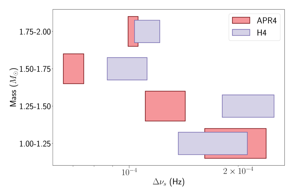
Figure 3 (figure 8 in the paper): This shows the size of a pulsar glitch that could be detected at 50% efficiency by our analysis. This is calculated with reference to a Vela-like pulsar — i.e. considering a fixed distance of 287 parsec and a spin (rotation around the neutron star’s own axis) frequency of around 11 Hz. The horizontal spread of the boxes represents the variation in the size of pulsar glitch when the different possible mass ranges for the neutron star, as shown on the corresponding vertical axis, is taken into account. Two extreme equations of state are considered: soft (APR4) and hard (H4). More details about these two different equations of state can be found in the scientific publication.
Find out more:
- Visit our websites:
- Read a free preprint of the full scientific article here or on arxiv.org.