Core-Collapse Supernovae (CCSNe) are spectacular deaths of massive stars with masses larger than 8 times the mass of our Sun (or, 8 solar masses). These stars burn hydrogen in their cores over millions or billions of years, in the process creating heavier elements up to iron. The iron builds up until it creates a so-called iron core in its center. When such an iron core is around 1.5 solar masses, its gravity becomes so strong that it exceeds the electron pressure of atoms and the star’s core collapses under its own weight. Under that tremendous pressure, the electrons penetrate the iron atoms, interacting with protons to create neutrons and neutrinos. The neutrons stay in the star’s core, but the very light neutrinos leave the collapsed core en masse. This massive flux of neutrinos is believed to drive the inevitable explosion of the star by heating it from the inside.
Targeted CCSNe
In our paper we describe a search for gravitational-wave (GW) transients focusing on CCSNe recorded by astronomical observations at distances up to approximately 20 megaparsecs (Mpc) (about 65 million light-years) during LIGO’s first and second observing runs, O1 and O2. We selected five CCSNe known by astronomers to have occurred during O1 and O2, to search for corresponding gravitational waves in archived O1 and O2 data: SN 2015as, SN 2016B, SN 2016X, SN 2017eaw and SN 2017gax.
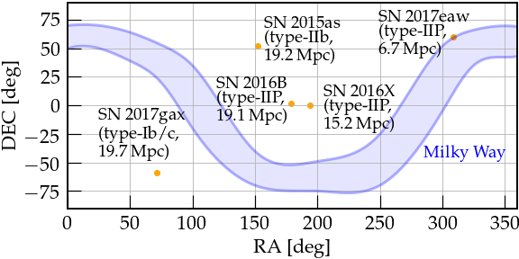
Figure 1: Sky locations of core-collapse supernovae analyzed inthis search. All were recorded within 20 Mpc during the O1 and O2 observing runs.
We expect a burst of gravitational waves to be emitted during a star’s iron core collapse. The collapse and massive flux of neutrinos trigger a shock-wave that leads to an explosion that reaches the star’s surface seconds to days later, depending on the size of the progenitor star. Unfortunately, the actual time when these collapses occurred is not known. Because of varying weather conditions on Earth, limited sky coverage of different optical observatories, and other obstructions, astronomical surveys do not typically find CCSNe until hours or months after the light from the event first reaches Earth. Extrapolating backwards in time to determine the moment of core-collapse depends primarily on how quickly a CCSN is observed by astronomers, the date of its last non-detection (i.e., the last time the galaxy hosting that supernova was imaged but the supernova was not present), and the properties of the progenitor (parent) star. We need to know when the CCSNe first appeared on the sky so we can search for any associated gravitational-wave signals from these events in LIGO data.
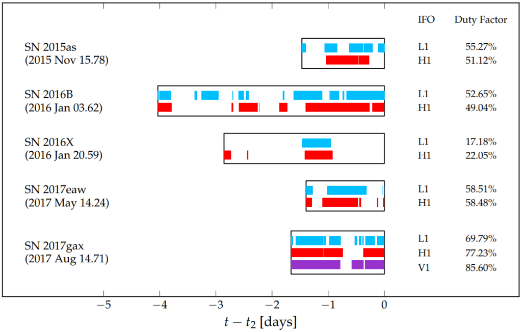
Figure 2: The time periods for each supernova where we expect to detect GW transient and the data we have available.
Supernova models
People have been observing supernovae for millennia, but the main mechanism behind these powerful explosions is not yet fully understood. Theorists model supernovae and calculate what gravitational-wave signals, or waveforms, from these events would look like. We then use those predictions to tune the search pipeline (e.g., all our signals are less than around 1s long, so anything longer than that is not considered a GW signal from a supernova) and estimate how far away we can detect such sources. In other words, we use models to teach our computers what signals to look for in the data. We then divide these simulated waveforms into two sets according to their explosion mechanisms.
The first set includes neutrino-driven explosion mechanisms for non- or slowly-rotating progenitor stars (see an example simulation). This set includes three waveform families, which differ from each other by variations in the approximations of conditions of the progenitor star, e.g., the influence of gravity, neutrino interactions within the star, and so on. In this scenario, heating by escaping neutrinos plays a crucial role in creating a supernova explosion. During the the initial stages, gravitational waves (GWs) are emitted in the frequency range from 100-300 Hz, while at later times, GWs up to around 2 kHz can be expected. The typical duration for a GW signal from one of these events is 0.5-1 s.
The second set of waveforms utilizes a magneto-hydrodynamically-driven (MHD-driven) explosion mechanism for rapidly-rotating progenitor stars. The magnetic effects related to the rapid rotation may play a dominant role in creating MHD-driven explosions. It is similar to a power generator: the faster a rotor spins, the more power it generates. However, almost all (99%) explosions are believed to come from slowly-rotating progenitor stars.
Along with these more realistic simulated CCSN explosions, we also consider two so-called extreme emission models. In one, the Long-Lasting Bar Mode model (see example video), we assume that the very rapid rotation (faster than the fastest observed pulsars) of the star deforms the collapsed core into a cigar- or a bar-shape. That rapidly spinning bar generates GWs. In the other extreme scenario, the Torus Fragmentation Instability model, we assume that a central black hole is created after the initial collapse. In this scenario, a torus (donut shape) of falling matter gets fragmented leading to large asymmetry in the torus. Such rapidly rotating clumps would emit GW. These scenarios are unlikely to occur, but they are not ruled out by astronomical observations.
Search results
In the first stage of our study we estimated how often random ‘noise’ in the LIGO detectors may produce apparent signals that are similar to real gravitational-wave signals. This is called a background analysis. Every physical experiment has to take into account a background. For example, if we want to measure how much light a bulb is emitting, we first measure the amount of light when the bulb is turned off (this is our background measurement), then we measure the amount of light emitted when the bulb is turned on. We then subtract one value from the other. In the GW background analysis, we first must analyze data that certainly are not GWs. If we look at the data from our detectors, any coincidence that we find between them may or may not be a real GW. To obtain a set of results that certainly are not GW signals, we artificially shift in time the data from one detector with respect to another. Because GWs travel at the speed of light, their maximum travel time between the LIGO Hanford and LIGO Livingston detectors is 10ms. And since the duration of the real GW signals could be 0.5 to 1 second long, any correlation of apparent signals in the detectors that is found when we shift the data in time by one second or more cannot be a gravitational wave.
After conducting the background analysis, we looked at the original, non-shifted data and assumed that the most energetic event, i.e., the loudest event, was a gravitational-wave candidate. Using this technique, so far we have not found any evidence for a gravitational-wave signal associated with our sample supernovae. All of the loudest events detected in this way were consistent with detector noise.
Since the background analysis did not reveal any CCSNe gravitational waves, we proceeded with constraining our understanding of CCSN engines.
Recalling that we trained our search pipelines to look for signals matching those that CCSNe models predict should occur, we added those predicted signals to the detector noise at different amplitudes corresponding to a potential supernova and ran the analysis again to see if we detected those signals. This allows us to see how often we could possibly pull such signals out of the background noise.
For example, imagine a supernova exploded at the distance of the Galactic center (about 30,000 light years). If we add 100 SN signals to the noise (at different times) and our search through the data only recovers 50, then we know that a real signal is detectable 50% of the time. Figure 3 illustrates some ‘detection efficiency’ curves that inform us how well we can detect different waveforms depending on how far away a supernova explodes. We derived detection efficiency curves as a function of distance for all supernova models used in our search. For neutrino-driven explosions, the detection distance reach is less than 5 kiloparsecs (kpc), or 16,300 light years. In the case of the more energetic MHD-driven explosions, the detection range reaches the distance of the Large Magellanic Cloud, at 50 kpc, or 163,000 light years. The situation is much different for the extreme emission models (those with the cigar-shaped core or asymmetric torus surrounding a black hole), which have ranges up to 28 megaparsecs (91 million light years).
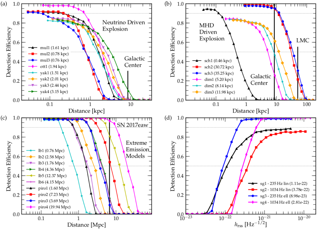
Figure 3: Detection efficiency curves for the models we use in the search. See text for more explanation.
The distance reaches for the extreme emission models cover the distances of the five specific supernovae we were looking for. Given that we did not detect them in LIGO data, we concluded that these ‘extreme’ models do not correctly describe the mechanism responsible for these known supernovae (otherwise, we should have detected something). Therefore, we exclude the parameter space of these models. We also concluded that if the deformation of the core happens inside a star due to rotation, that deformation is too small and short-lived for us to detect a GW from it. Alternatively, if a black hole is created inside a star and a clump of matter accretes into that black hole, this clump is also too small to generate a GW we can detect.
Our analyses also provided constraints on the GW energy emission from CCSNe. This is the minimum energy emitted in gravitational waves needed to be detectable in 50% of cases. We assume that the dominant gravitational-wave emission is either at low or high frequencies. We found out that at low frequencies, our energy constraint is around 0.0001 solar masses times the speed of light squared (since the energies are so large, we use the equation E=mc2 to express these energies), which is about the explosion energy typically observed by astronomers. At high frequencies, the energy constraint is two orders of magnitude less stringent than for low-frequency emission. These constraints can allow us to better understand the supernova engine (e.g.: qthe larger the asymmetry of the explosion, the larger the emitted energy). So far, the values we have obtained are not yet informative, but we will continue searching.
Read more
- Visit our websites: https://ligo.org, http://www.virgo-gw.eu
- Full scientific article: An Optically Targeted Search for Gravitational Waves emitted by Core-Collapse Supernovae during the First and Second Observing Runs of Advanced LIGO and Advanced Virgo, submitted to Phys. Rev. D. Free arXiv preprint: arXiv:1908.03584 [gr-qc]
- Previous article on this topic: A First Targeted Search for Gravitational-Wave Bursts from Core-Collapse Supernovae in Data of First-Generation Laser Interferometer Detectors Phys. Rev. D 94, 102001 (2016). Free arXiv preprint: arXiv:1605.01785 [gr-qc]