Discovering gravitational waves from coalescing binary black holes
The Advanced LIGO (aLIGO) detectors first observed gravitational waves as a characteristic chirp in the data, named GW150914. By comparing the data to solutions of Einstein’s theory of gravity, we realized the data agreed with what we expected from the coalescence of two stellar mass black holes. To read more about the discovery and initial interpretation of GW150914, visit the associated science summary pages.
But we like to be sure. Einstein’s equations are hard to solve, so our initial interpretation relied on models designed to extend the knowledge gained by careful, systematic, but necessarily approximate solutions. Here we summarize a reanalysis of GW150914 by a different method than the one we used the first time. In this case, we directly compare the data to supercomputer simulations of binary black hole motion.
What did we do?
Solving Einstein’s equations on a supercomputer
The process of solving Einstein’s equations on a supercomputer is called numerical relativity. Our detailed understanding about the coalescence of binary black holes comes, in the end, from numerical relativity simulations. However, these simulations are notoriously challenging, requiring weeks to months of time on the world’s fastest supercomputers. Working with four teams of experts in numerical relativity (RIT, SXS, Georgia Tech, and the BAM team), we assembled a large collection of more than one thousand simulations of binary black holes.
Scaling supercomputer simulations to GW150914
In the original analysis of GW150914, which you can read about here, we compared the data to simple models for the gravitational waves from coalescing binary black holes. Using these models, we could perform the comparison millions of times, for any kind of binary black hole the models allowed. In this new analysis, however, we restricted ourselves to only compare the data to the roughly one thousand simulations described above.
Fortunately, because Einstein’s theory of gravity works the same way for all objects, no matter their mass, we can scale each simulation to larger or smaller black holes. In other words, for every simulation, we can pick any total binary mass we want. Still, we only have one thousand simulations to cover all the other parameters needed to describe a binary black hole, such as the ratio between the two black hole masses and the spins of the black holes.
Nature has been kind, however: GW150914 looks incredibly similar to the majority of simulations performed to date, the last few orbits of similar-mass binary black holes. Of the thousand simulations, we knew that many could be scaled to resemble the data.

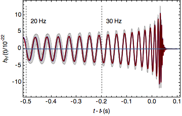
Figure 1: This image shows the gravitational waves reconstructed from GW150914. We measure a 90% probability that GW150914’s strain, shown on the vertical axis, lies inside the shaded region. The solid lines show the predictions of numerical relativity.
Putting the puzzle back together
The problem of reconstructing the black hole’s properties turns into a jigsaw puzzle: we have only some of the pieces, but from experience we know the picture was drawn with a broad brush. We can boil the comparison between the data and a particular simulation and mass down to one number. This number (referred to as the marginalized likelihood) tells us the color of each piece of the puzzle. For an object like GW150914, with very few gravitational wave cycles, the colors of neighboring pieces of the puzzle are necessarily similar. So even though we’re missing most of the pieces, we can still figure out what the whole puzzle looked like. Or, at least, the most important part of the puzzle: the part that describes black holes most like GW150914. Figure 2 shows an example: with only a few points (simulations), we can figure out the appropriate color (likelihood) to use in any place on these three panels.

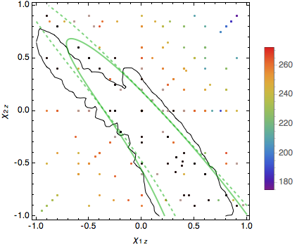
Figure 2: The colored dots in these figures show the location of numerical relativity simulations. The colors indicate the results of comparing them to the data. The colors change smoothly: we can estimate the appropriate color to use even in places where no simulations exist.
Why does it matter?
In our original analysis, which you can read about here, we were excited to identify the masses and spins of the two black holes. These provide pieces of another jigsaw puzzle: how do we make binary black holes in the first place?
Our new analysis teased out a little more information about the two black holes that merged to form GW150914, using information uniquely available from numerical relativity simulations. Perhaps most importantly, our conclusions were similar to those of the original analysis, proving that our results are robust.
This work also more explicitly illustrated a result we learned in our initial interpretation of GW150914: how binary black holes with very different dynamics can, under suitable circumstances, produce gravitational waves like GW150914. Some of the simulations which fit the data were simple, with the inspiral occurring entirely within one plane. In others, the orbital plane slews strongly (or precesses) through the merger. The movies below illustrate the range of possible sources of GW150914.

Figure 3: The green curves in this image show which combinations of black hole spins are consistent with the data, in units of the maximum possible spin. We found the green curve by using (and connecting) the colors on the dots. The solid black curve is the result we found in our first analysis of GW150914. (This figure assumes the binary’s orbit remains in the same plane.)
Finally, by measuring how similar each simulation was to this event, we can now figure out where new simulations would fill in the gaps, for this and future events.
Read more:
- The publication reporting a direct comparison between GW150914 and numerical relativity
- The publication reporting the parameter estimation of GW150914
- The publication reporting the discovery of GW150914
- Another publication reporting an initial comparison of GW150914 with numerical relativity
- Introductions to numerical relativity:
- Physics Today article (Baumgarte and Shapiro)
- Review articles: Sperhake 2015 and Centrella, et al. 2007
- Textbooks: Baumgarte and Shapiro, Alcubierre
Watch more:
The four groups have made movies of the dynamics of GW150914-like black hole binaries, based on their simulations:
- YouTube movie from Georgia Tech (not precessing)
- YouTube movie from SXS (not precessing)
- YouTube movie from RIT (precessing)
- YouTube movie from UIB (precessing)

